Theory
This section discusses the theory used in the Public Transport program:
Generalized cost is a measure of the main components of a Public Transport trip. The generalized cost of a public transport trip has three components:
Time
Inconvenience
Cost
The route-evaluation process considers each component separately. The route enumeration process, described in Route enumeration cost calculation, uses a slightly simpler estimation.
A trip’s generalized cost automatically includes walk and in-vehicle time; the cost might include wait time, boarding and transfer penalties, and fare, depending on the values of keywords in the FACTORS control statement.
Generalized cost is a linear function of its components, weighted by coefficients. The coefficients let you:
The Public Transport program measures generalized cost in time, using minutes as the s working units. Fares, if used, are input in monetary terms and converted into the corresponding time units.
Subsequent sections provide details about individual components and their weighting factors.
Walking may occur at the following points in a trip:
-
Between stop node and zone centroid, at the start and end of the trip
-
Between stop nodes, as part of a transfer between services
-
Between an origin and destination zone, without using any transit mode
You can develop walk links outside the Public Transport program and input the links to the program, or you can develop the walk links when developing the public transport network.
A link’s walk time (nontransit time) is typically the actual travel time. To convert the times to perceived values (for inclusion in generalized costs), you can weight the link times with the RUNFACTOR keyword.
The program uses the combined headway of available transit services to compute the wait time at any boarding point. Specifically, the program computes wait time from wait curves that you specify. If you do not specify any wait curves, the program uses default wait curves. To represent passengers’ ability to control wait time at the start of a trip but not at transfer points, you may specify different wait curves for initial and subsequent boardings at each node.
You define wait curves with the WAITCRVDEF control statement. You assign wait curves to nodes with IWAITCURVE and XWAITCURVE keywords in the FACTORS control statement. You can weight the wait times with the node-specific WAITFACTOR keyword.
The program uses default wait curves at nodes where you do not assign wait curves. See Default wait curves for a description of the default wait curves.
When the program performs crowd modeling with wait time adjustments, passengers might experience additional wait time attributable to crowding. For example, a transit service might be so loaded that a passenger cannot board (and must wait for a later service). Similarly, a network bottleneck might occur (where demand exceeds capacity, and some passengers cannot proceed forward within the modeled period). You model these additional wait times with a node-specific WAITFACTOR keyword in the FACTORS control statement.
In-vehicle time is the time passengers spend travelling in a public transport vehicle for each transit leg of a trip. If a trip has more than one leg, the value is the total in-vehicle time for all legs.
You can weight in-vehicle time with a transit-mode-specific value specified with the RUNFACTOR keyword.
When performing crowd modeling with link travel-time adjustments, the program also weights in-vehicle time with a crowding factor.
Boarding penalty is a fixed penalty applied at each boarding (that is, at the start of the trip) and at each interchange. You may specify separate penalties for each mode. The default penalty for each mode is zero (that is, no penalty).
You specify boarding penalties by mode with the BRDPEN keyword.
Transfer penalty is the transit-mode-to-transit-mode interchange penalty, which represents the inconvenience of transferring between modes. The program applies this penalty at transfer points, even if there is walking between the two modes. The penalty is based on a combination of alighting and boarding modes.
The transfer penalty applies in addition to the boarding penalty for the subsequent transit leg. For transfers between the same mode, you might set the transfer penalty to a negative value to counteract or reduce the boarding penalty applied to the subsequent leg of that mode.
You can ban changes between modes by setting a high transfer penalty, such as 999, for that mode-to-mode combination. All mode-to-mode penalties default to zero—that is, there are no penalties by default.
You specify transfer penalties with the XFERPEN keyword. You may add constants to transfer penalties with the XFERCONST keyword, and you may weight transfer penalties with the XFERFACTOR keyword.
By defining fare models, you can include fares in the route- evaluation and skimming processes. Fare models describe how the program computes the fare for part of a trip or for an entire trip.
You define fare models with the FARESYSTEM control statement, and specify the input file with the FILEI control statement and FAREI keyword.
You associate fare models with transit lines two ways:
-
Directly with the LINE statement and FARESYSTEM keyword
-
Through their mode or operator attribute, with the FACTORS control statement and FARESYSTEM keyword
Route enumeration cost calculation
Route enumeration is a heuristic process that identifies a set of discrete routes between zone pairs along with the probability that passengers will use the routes to travel between the zones.
Data compression techniques improve the performance of the route-enumeration process. For example, the process bundles together transit legs with the same boarding and alighting points, and enumerates routes only for the cheapest leg in the bundle. (The process disaggregates transit leg bundles for analysis.) For this reason, the process cannot use all the components of generalized cost.
The route-enumeration process converts the following components to generalized cost units:
-
In-vehicle time, weighted by mode-specific factor specified with the RUNFACTOR (using the value of the bundle’s fastest transit line)
-
Boarding penalty
-
Wait time, weighted by WAITFACTOR and subject to a range defined by REWAITMIN and REWAITMAX
The route-enumeration process uses a simple estimate of wait time for each leg bundle. The process computes the headway for each bundle’s boarding node from the sum of the frequencies of the bundle’s legs. The process sets the wait time to half this headway, weighted by WAITFACTOR. Where necessary, the process adjusts the resulting value to fall within the range set by REWAITMIN to REWAITMAX. You can exclude wait time from the route-enumeration process by setting these factors to zero.
-
Walk time, taken directly from nontransit legs and weighted by an appropriate RUNFACTOR
When modeling best paths (or when REBESTPATHCOST is T), the route-enumeration process handles some of these components differently. In this case:
-
Calculations of wait and in-vehicle time depend on the value of FREQBYMODE:
When true (default value), the process computes these times for individual modes (and the value for fastest mode subsequently used in enumeration).
When false, the process computes these times across all modes in a transit leg bundle.
-
In-vehicle time is based on the average value for lines in the transit leg bundle. The process uses the calculations described in SFM and SFCM examples to discard any slow routes in the bundle and to obtain the required value.
-
Wait time is calculated using initial or transfer wait curves and WAITFACTOR (as in the route-evaluation process). The process uses the headway of the transit-leg bundle (or the lines of a particular mode in the bundle) after discarding any slow routes. For best-path models, the route-enumeration process uses transfer penalties (based on XFERCONST, XFERFACTOR, and XFERPEN) when identifying discrete routes.
The route-enumeration process does not consider fares, and ignores transfer penalties except when modeling best paths. Instead, the route-evaluation process disaggregates transit-leg bundles by mode to apply transfer penalties. Using fares and transfer penalties with leg bundles during route enumeration could eliminate valid routes. For example, consider a banned transfer between transit modes 3 and 5. Routes transferring from a mode-3 leg to a mode-5 leg would be eliminated. However, suppose these legs are the top legs in bundles that contain legs of other modes. These other legs would also be eliminated.
The route-enumeration process adds wait time to the time of each bundle’s top leg to obtain a transit-leg cost.
The report produced by the TRNLEGS3 keyword in the REREPORT control statement shows the generalized cost of transit legs used during the route-enumeration process.
This section discusses the algorithms that the Public Transport program uses. The program supports two distinct modeling methods: multirouting and best-path. For both modeling methods, the program finds attractive or reasonable routes, (that is, routes that have some probability of use), in three steps: network simplification, route enumeration, route evaluation. You can restrict modeling to consider just those routes that use a particular transit mode at some stage in the trip.
This section discusses:
Multirouting and best-path methods
During a public transport trip, passengers must make decisions at several points on their route. When on a transit line, passengers might need to decide which stop to alight at (in order to transfer or walk to their destination). At the origin and on completion of a transit leg, passengers must decide where to board the next transit leg. At a stop, passengers must choose between the transit lines that enable progress toward the destination.
A number of possible methods, or modeling philosophies, are possible at each decision point. The Public Transport program includes two distinct methods:
-
Multirouting — Evaluate multiple routes and calculate the probabilities of using each one.
-
Best-path — Identify a single "best path" route for an origin- destination pair.
For example, suppose travelers waiting at node N have a choice between two routes to reach the trip’s destination. The first route uses line L, which runs every 20 minutes and takes 15 minutes to reach the destination after boarding. The second route uses line M, which runs every 30 minutes and takes 11 minutes to reach the destination. Either line offers an efficient effective route towards the required destination. Taking these values as components of the generalized cost (without need for further weighting), you can compute an expected travel time from the stop to the destination.
In a multirouting model, travelers are prepared to board whichever bus comes first. There are a total of five services per hour. Assuming equal spacing of departures, the combined headway is 12 minutes and average wait is 6 minutes. The cost to the destination is the wait time plus travel time, either 11+6 or 15+6, that is, 17 or 21. Assuming route usage proportional to service frequency, the average time to destination is 19.4 minutes.
In a best-path model, travelers choose between the two routes and then wait for a service on the chosen transit line (ignoring any service on the other line). Travelers assess attributes of each route: L has an average wait of 10 minutes and travel time of 15 minutes, for a total cost of 25 minutes. M has an average wait of 15 and travel time of 11, for a total of 26 minutes. Therefore, travelers using the best-path method would select transit line L, with an average trip cost of 25 minutes.
Model developers must decide between the two methods. The appropriate method might depend on externally imposed requirements or practices (for example, guidelines from government departments) or a choice regarding the suitability of each method. Many modelers prefer the multirouting method in cities with extensive, well-developed public transport systems.
To improve performance and to minimize memory and storage requirements, the Public Transport program simplifies the public transport network into a set of intermediate data structures:
See Network simplification for a description of these data structures.
For multirouting modeling, the route-enumeration process finds all potentially attractive routes and enumerates them. The process follows three principles:
-
The trip should move progressively from the origin to the destination.
-
Travelers prefer simpler trips, that is, direct trips or trips that involve few transfers.
-
Travelers are unwilling to walk very long distances.
The route-enumeration process uses these principles to identify reasonable routes.
First, the process establishes connectivity between transit lines. This step is analogous to travelers examining a map and identifying the sequence of lines they can use to travel from their origin to their destination. The process limits routes by choosing simpler trips and trips with shorter walking distances during line-to-line transfers.
Next, the process identifies the route attributes—basic cost and number of transfers—and compares them, selecting reasonable routes for evaluation. This step is analogous to travelers rejecting routes that are very long relative to more direct alternatives.
For best-path modeling, the route-enumeration process identifies possible routes for the best single path between an origin and a destination. The route-enumeration process uses the same cost components as the route-evaluation process, with the exception of transfer penalties. The route-enumeration process allows for possible transfer-penalty values, and enumerates any route which potentially could be the best route.
See Route-enumeration process for a detailed description of this process.
For multirouting models, the route-evaluation process takes the explicit list of reasonable routes between an origin and destination and determines which routes passengers will use to make trips and what fraction of passengers will use each route.
The route-evaluation process treats the routes like a hierarchy of conditional choices: Each stop or branch point represents a decision whether to board a service, alight from a service, or walk elsewhere to board another service. The program uses conventional algorithms to forecast these individual choices. For example, the program uses information about the trip sequence to preclude alighting and reboarding the same service.
For best-path models, the route-evaluation process identifies the best path using a similar evaluation method, and assigns all demand to that route.
Limiting selected routes to particular transit modes
The Public Transport program uses the route-enumeration process to identify possible routes from an origin to a destination, followed by a the route-evaluation process to evaluate the routes. The enumerated routes may vary widely in characteristics, perhaps having different transfer points, and using different modes.
Sometimes you might want routes to use a particular mode. Earlier software packages used biases to attract travelers toward one mode and away from other modes. However, biasing could lead to modeling distortions affecting route costs or identification of the best route.
With the Public Transport program, you need not use biases. Instead, you can specify a "must-use-mode"—a mode that must be used during at least one leg of a public transport route in order for the Public Transport program’s route-enumeration process to select that route.
Advantages of the Public Transport program for multirouting
Some software packages trace paths from all zones to a particular zone or vice-versa. Such paths do not retain the history of a trip at a node (that is, how the path reached the node or where the path came from). When using multiroute paths, such packages cannot easily extract route-based information, such as station-to-station movements, matrices of trips using selected links or transit lines, or mode-to-mode and operator-to-operator transfers.
The Public Transport program finds discrete multiple routes between pairs of zones. Therefore, unlike traditional software packages, the Public Transport program operates at the zone-pair level rather than at the zonal level. The Public Transport program requires more computational time but produces more useful and better quality results.
The Public Transport program addresses other common problems associated with multirouting:
-
Calculating wait time at stops using the combined frequency of visiting services
-
Modeling access, egress, and transfer choices
-
Modeling combination of frequent and infrequent services
Public transport networks are often quite detailed and data intensive. To improve algorithm performance and minimize memory and temporary disk storage, the Public Transport program simplifies the network for enumerating and storing routes. The program stores the simplified network in intermediate data structures, which you can examine to gain an understanding of how multirouting works in the Public Transport program.
Use the DELMODE, DELACCESSMODE, and DELEGRESSMODE factors to remove legs of particular modes from the network representation. The program does not use specified legs at any stage in the modeling.
This section introduces the network representations used for:
A transit leg is a trip segment, from a boarding point to an alighting point, that uses a single transit line. Travel on the transit line can be over one or more links in the public transport network. (A trip consists of an access leg, and one or more pairs of transit leg bundles and nontransit legs, the last of which is the egress leg.)
Use the REREPORT control statement and LINES keyword to produce a line-attribute report.
Line-attribute report
REPORT: LINES
Int                           Fare #Line #Stop  Line
Line#   DIR  Mode   OP  HDWAY Type Nodes Nodes  Name
----------------------------------------------------
20    (f)   7   11    5.00    0    10     5  GMB1-1B

                Dis-   Line   Stop
    Node   Time   tance  Node#  Node#
--------------------------------------
     727   0.00    0.00      1      1
    -897   0.28    0.12      2      0
    -947   0.97    0.42      3      0
     875   1.99    0.80      4      2
     751   5.54    1.15      5      3
    -881   6.36    1.55      6      0
     748   7.10    1.92      7      4
    -745   8.40    2.39      8      0
    -746   12.33   4.16      9      0
     747   19.15   7.08     10      5
Use the REREPORT control statement and TRNLEGS3 keyword to produce a line-ordered transit-leg report.
Sample transit-leg report for the GMB1-1B transit line
REPORT: TRANSIT LEGS III (Legs for Lines)
(REnum Time = actual time * RUNFACTOR + BRDPEN)

Int                           Fare #Line #Stop Line
Line#  DIR  Mode    OP   HDWAY Type Nodes Nodes Name
---------------------------------------------------
    20   (f)     7    11    5.00    0    10     5 GMB1-1B

Top    ON        OFF    Time    Time    Dis-
Leg    Node     Node    Actual  REnum   tance
----------------------------------------------
        727      875      1.99   4.99    0.80
        727      751      5.54   8.54    1.15
        727      748      7.10  10.10    1.92
*       727      747     19.15  22.15    7.08
        875      751      3.55   6.55    0.35
        875      748      5.11   8.11    1.12
*       875      747     17.16  20.16    6.28
        751      748      1.56   4.56    0.77
*       751      747     13.61  16.61    5.93
*       748      747     12.05  15.05    5.16
* Top leg of a leg bundle, see Transit-leg bundles.
A transit-leg bundle is a collection of transit legs that use different transit lines but board and alight start at the same node. Transit-leg bundles have the following properties:
-
The "top leg" of the bundle is the cheapest in terms of travel time (in the example all legs within bundles have the same time).
-
They may or may not traverse the same links of the underlying network.
The route-enumeration process treats transit-leg bundles as single entities, thus simplifying and reducing the data to examine and enumerate. The program individually evaluates each leg within a transit-leg bundle when determining "attractive" routes for loading and skimming.
Use the REREPORT control statement and TRNLEGS2 keyword to produce a node-ordered transit-leg-bundle report.
Excerpt from node-ordered transit-leg-bundle report
REPORT: TRANSIT LEGS II (Leg Bundles from Nodes)
(REnum Time = Actual Time * RUNFACTOR + BRDPEN)
(And top leg in Bundle includes Estimated Wait time for Bundle)
Top      ON    OFF     Time    Time    Dis-    Line
Leg    Node   Node   Actual   REnum   tance    Name
---------------------------------------------------
*       875    753     5.03    6.03    0.83    GMB1-24MA
        875    753     5.03    5.53    0.83    PLB1-113A
        875    753     5.03    5.53    0.83    PLB129A
        875    753     5.03    6.04    0.83    RES-903R
*       875    757     5.32    6.32    1.06    GMB1-24MA
        875    757     5.32    5.85    1.06    PLB1-113A
        875    757     5.32    5.85    1.06    PLB129A
        875    757     5.32    6.38    1.06    RES-903R
*       875    765     6.30    9.30    1.66    GMB1-24MA
*       875    774     7.75    10.75   1.95    GMB1-24MA
*       875    773     8.26    11.26   2.35    GMB1-24MA
*       875    776     13.04    16.04  4.30    GMB1-24MA
*       875    778     17.37    20.37  5.97    GMB1-24MA
*       875    751     3.55    4.55    0.35    GMB1-2B
        875    751     3.55    3.55    0.35    GMB1-24MA
        875    751     3.55    3.55    0.35    GMB1-1B
        875    751     3.55    3.91    0.35    PLB1-113A
        875    751     3.55    3.91    0.35    PLB129A
        875    751     3.55    4.26    0.35    RES-903R
*       875    748     5.11    7.36    1.12    GMB1-2B
        875    748     5.11    5.11    1.12    GMB1-1B
This sample shows transit legs from node 875, including three sets of leg bundles: from node 875 to nodes 753, 757, and 751. When multiple lines connect node 875 to an alighting node, the report marks the top line (the fastest line or the first line, if all have equal time) with "*". All legs in a bundle have the same actual in-vehicle time, but the REnum time for the bundle’s top leg includes an estimate of the bundle’s waiting time. (Do not confuse this waiting time with the wait time calculated during the route-evaluation process. See Generalized cost.)
Nontransit legs are minimum-cost segments, traversed by nonmechanized modes. Nontransit legs connect:
-
Zones and stop nodes or stop nodes and zones that allow access to and egress from the transit system
-
Two stop nodes that allow a transfer between two lines
Nontransit legs may traverse none (special case), one, or multiple physical links. The program derives leg attributes from link attributes.
The program can generate nontransit legs with the GENERATE control statement, input user-specified nontransit legs, or do both. The program associates a cost with these nontransit legs.
The program automatically generates a third type of "notional" nontransit leg, which allows transfers between two lines visiting the same node. Such nontransit legs do not have any associated cost.
Boarding and transfer costs apply to both types of transfers—those occurring at a node and those between two nodes connected with a physical nontransit leg.
Use the REREPORT control statement and ACCESSLEGS, EGRESSLEGS, and XFERLEGS keywords to produce nontransit-leg reports.
Sample nontransit-leg report: REREPORT ACCESSLEGS
REPORT: ACCESS LEGS
         Desti-          Dis-
Origin   nation   Time   tance  Mode
----------------------------------------
     1      773   2.56    0.25    33
     1     2052   8.70    0.36    33
     1     3674   2.70    0.18    33
     2      778   1.36    1.06    33
     3      749   3.12    0.78    33
     4      750   0.40    0.31    33
     4      875   1.52    0.32    33
     4     2004   7.52    0.41    33
     5      959   2.70    0.11    33
     6      796   1.92    0.38    33
     6      800   1.92    0.39    33
     6     2054   5.40    0.53    33
     6     2056   5.92    0.43    33
Sample nontransit-leg report: REREPORT EGRESSLEGS
REPORT: EGRESS LEGS
         Desti-          Dis-
Origin   nation   Time   tance   Mode
----------------------------------------
   703       19   0.64    0.23     33
   705       19   0.96    0.19     33
   709       19   0.96    0.70     33
   714       20   1.32    0.22     33
   716       20   1.80    0.24     33
   721       21   1.68    0.42     33
   725       22   6.00    0.24     33
   728       22   0.52    0.36     33
   730       22   0.76    0.20     33
   734       22   0.80    0.30     33
   735       23   2.64    2.46     33
   747       24   1.72    0.43     33
   749        3   3.12    0.78     33
Sample nontransit-leg report: REREPORT XFERLEGS
REPORT: TRANSFER LEGS
         Desti-          Dis-
Origin   nation   Time   tance   Mode
----------------------------------------
   701      701   0.00    0.00     -1*
   702      702   0.00    0.00     -1
   703      703   0.00    0.00     -1
   800      800   0.00    0.00     -1
   800     2056   4.00    0.04     34
   803      803   0.00    0.00     -1
   806      806   0.00    0.00     -1
   806     2058   4.00    0.27     34
   813      813   0.00    0.00     -1
   813     2060   4.00    0.16     34
   823     2062   4.00    0.11     34
   830      830   0.00    0.00     -1
   830     2066   4.00    0.02     34
   837      837   0.00    0.00     -1
   838      838   0.00    0.00     -1
   838     2072   3.00    0.11     34

* -1 indicates a direct transfer, without any walking.
During network simplification, the program expands access and egress nontransit legs—legs from zone to stop node and vice versa—into zone to line and line to zone legs. The program stores line-zone legs as pointers to the corresponding access and egress nontransit legs along with some additional information that helps improve the performance of the route-enumeration algorithm.
When multiple access and/or egress legs exist between a zone and a line, the program might eliminate some legs or restrict their use to ensure that routes starting or terminating on a line use distinctive segments and do not overlap. For best-path models, the program uses all connectors to ensure identification of the best route; because the program selects exactly one best route, overlapping segments are not possible.
For multirouting models, the program eliminates multiple access legs by applying the following rules:
-
Among a set of legs accessing consecutive stops (disregarding intermediate nonstopping nodes), select the leg with the least generalized cost and discard the others. (Between legs of equal cost, select the downstream leg.) If SHORTESTWALK=F then selection is based on lowest travel time to some downstream point on the line (rather than shortest leg cost).
-
Always retain the first access leg (that is, the leg connected to the transit line’s earliest stop).
-
If the cost of the "first access + riding to the next" is more than the cost of the next access, those boarding at the first access may only ride until the stop before the next access.
-
If the cost of the "first access + riding to the next" is less than the next access, discard the next access.
-
Each access has a stop up to which those boarding can ride; either to the stop before the next valid access or to the end of the line.
For multirouting models, the program eliminates multiple egress legs by applying the following rules:
-
Among a set of legs providing egress from consecutive stops (disregarding intermediate nonstopping nodes), select the leg with the least generalized cost and discard the others. (Between legs of equal cost, select the upstream leg.) If SHORTESTWALK=F then selection is based on travel time from some upstream node on the line.
-
Always retain the last egress leg (that is, the leg connected to the transit line’s latest stop).
-
If the cost of an egress leg is more than the cost of "riding to the next + next egress", discard the leg.
-
If the cost of the an egress leg is less than the cost of "riding to the next + next egress", then only those boarding after the current egress can use the next one.
-
Each egress has a stop that specifies the beginning of a range of valid boarding stops; this may be the stop after the previous valid egress or the beginning of the line.
Both sets of rules apply to circular lines.
Use the REREPORT control statement and LINEZONLEG1 LINEZONLEG2 keywords to produce line-to-zone nontransit-leg reports.
Sample line-ordered line-to-zone nontransit-leg report(REREPORT LINEZONLEG1)
REPORT: LINE ZONE I (In Line Order)
    Origin  Dest          Dis-    Access/  Line
    Node    Node   Time   tance   Egress   Name
-----------------------------------------------
        6    800   1.92    0.39   Access   GMB1-49MA
      800      6   1.92    0.39   Egress   GMB1-49MA
        7    803   1.52    0.41   Access   GMB1-49MA
      803      7   1.52    0.41   Egress   GMB1-49MA
        8    814   0.88    0.12   Access   GMB1-49MA
      814      8   0.88    0.12   Egress   GMB1-49MB
        3    749   3.12    0.78   Access   GMB1-2A
       22    728   0.52    0.36   Access   GMB1-2A
      728     22   0.52    0.36   Egress   GMB1-2A
      749      3   3.12    0.78   Egress   GMB1-2B
        4    875   1.52    0.32   Access   GMB1-2B
      875      4   1.52    0.32   Egress   GMB1-2B
       15    852   1.52    1.33   Access   GMB1-29AA
      855     16   1.80    0.97   Egress   GMB1-29AA
      852     15   1.52    1.33   Egress   GMB1-29AB
       16    855   1.80    0.97   Access   GMB1-29AB
Sample zone-ordered line-to-zone nontransit-leg report(REREPORT LINEZONLEG2)
REPORT: LINE ZONE II (In Zone Order)
    Origin  Dest          Dis-    Access/  Line
    Node    Node   Time   tance   Egress   Name
-----------------------------------------------
         1   773   2.56    0.25   Access   GMB1-24MA
         1   773   2.56    0.25   Access   GMB1-24MB
         1   773   2.56    0.25   Access   GMB1-36A
         1   773   2.56    0.25   Access   GMB1-36B
         1  2052   8.70    0.36   Access   ISL-UP
         1  2052   8.70    0.36   Access   ISL-DN
       773     1   2.56    0.25   Egress   GMB1-24MA
       773     1   2.56    0.25   Egress   GMB1-24MB
       773     1   2.56    0.25   Egress   GMB1-36A
       773     1   2.56    0.25   Egress   GMB1-36B
      2052     1   8.70    0.36   Egress   ISL-UP
      2052     1   8.70    0.36   Egress   ISL-DN
         2   778   1.36    1.06   Access   GMB1-24MB
       778     2   1.36    1.06   Egress   GMB1-24MA
         3   749   3.12    0.78   Access   GMB1-2A
       749     3   3.12    0.78   Egress   GMB1-2B
         4   750   0.40    0.31   Access   PLB1-113B
         4   750   0.40    0.31   Access   PLB129B
         4   750   0.40    0.31   Access   PLB127A
         4   750   0.40    0.31   Access   PLB127B
         4   750   0.40    0.31   Access   RES-91R
During network simplification, the program expands nontransit legs between stop nodes, direct transfers at the same stop node, and walk transfers between stops into line-to-line legs. The program stores line-line legs as pointers to the nontransit transfer legs along with some additional information that improves the performance of the route-enumeration algorithm.
The route-enumeration process eliminates some transfer legs. When generating line-to-line legs, the program applies the following rules:
-
For multirouting, among multiple connectors between consecutive stops on a "from-line" and consecutive stops on a "to-line", retain only the lowest-cost connector; discard the others. If SHORTESTWALK=F then the connector with shortest through travel time from an upstream node on the from-line to a downstream node on the to-line is selected (rather than the lowest cost connector).
-
Do not permit transfers from a transit line’s first node; passengers must use the line before transferring.
-
Do not permit transfers to a transit line’s last node.
-
For circular lines with the same first and last nodes, permit boarding at the first node and alighting at the last node.
-
For multirouting, prohibit transfers involving backtracking, such as if the node prior to alighting is the same as the one after boarding.
-
If two lines traverse the same physical route with the same stop characteristics, record only one transfer location for consecutive stops.
For example, consider the following transit lines.
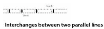
In this case, the program only records one transfer location between Lines A and B instead of four—the last stop. The program relaxes this restriction during route evaluation to give flexibility in transfer location, especially when modeling crowding.
However, if stop 2 is a stopping node for line A and not for line B, then the program records two transfer locations: one at stop 1 and one at stop 4 (representing transfers at stops 3 and 4). If two lines meet at nonconsecutive stops, diverging between them, the program records a transfer location at each stop where they meet.
Use the REREPORT control statement and LINELINELEG keyword to produce line-to-line transfer-leg reports.
Sample line-to-line transfer-leg report (REREPORT LINELINELEG)
REPORT: LINE TO LINE LEGS
   From/To  From/To   From/To
  LineNode  NodeSeq#  LineName
------------------------------
       799         7  GMB1-49MA
       799        14  PLB144A
       806         4  GMB1-49MA
       806         7  PLB144B
       806         4  GMB1-49MA
       806        34  PLB129A
       799         7  GMB1-49MA
       799        14  PLB129B
       806         4  GMB1-49MA
      2058        13  ISL-UP
       806         4  GMB1-49MA
      2058        16  ISL-DN
       800         6  GMB1-49MA
      2056        10  ISL-UP
       800         6  GMB1-49MA
      2056        19  ISL-DN
       799         7  GMB1-49MA
       799         1  GMB1-39MA
Route enumeration is a heuristic process that identifies a set of discrete routes between zone pairs along with the probability that passengers will use the routes to travel between the zones. Use keywords in the FACTORS and PARAMETERS control statements to control the route-enumeration process.
The program measures trip cost differently during route-enumeration than during route-evaluation. See Route enumeration cost calculation.
Route enumeration has three distinct stages:
The process varies only slightly when you specify a must-use mode. See Enumerating routes with a must-use mode specified. Public Transport also includes an option to enhance the stability of the process under small variations of input network characteristics. See Modified route enumeration process.
The route-enumeration process finds minimum-generalized-cost routes between zone pairs to establish a baseline cost. Each route has an access leg, and one or more pairs of transit and nontransit legs, the last of which is an egress leg. Using explicit couples of transit and nontransit legs is consistent with the multiroute-enumeration process, described in Enumerating routes.
Because the process starts with transit-leg bundles rather than individual transit legs, the process might disaggregate a minimum-cost route into one or more discrete routes. For example, the following minimum-cost route is a collection of 14 individual routes:
Route(s) from Origin 1 to destination 100
1 -> 1276
1276 -> 1572 -> 1583 lines 744 746
1583 -> 1654 -> 100 lines 399 476 478 486 489 493 495
where:
-
Node pair 1->1276 is the access leg from node 1.
-
Triplet 1276->1572->1583 represents a transit leg between node 1276 and node 1572 on line 744 or 746, and a nontransit-transfer leg between node 1572 and node 1583.
-
Triplet 1583->1654->100 represents a transit leg between node 1583 and node 1654 on line 399, 476, 478, 486, 489, 493, or 495, and an egress leg between node 1654 and node 100.
The route via lines 744 and 399 will have the best travel cost; the other routes may have the same or slightly longer vehicle travel time.
The route minimizes the generalized cost, not the number of transfers. Therefore, identified routes might have more than MAXFERS transfers. However, you can reflect the impact of transfers in the generalized cost with sensible boarding penalties.
You can specify a "spread", an upper cost limit for routes between an O-D pair when using multirouting. Select the function for calculating the spread with the SPREADFUNC keyword, and specify function parameters with the SPREADFACT and SPREADCONST keywords. The route-enumeration process uses the costs from the minimum cost routes and the spread to determine a maximum cost value for "reasonable" routes to that destination.
Similarly, to set the maximum number of transfers permitted on "reasonable" routes to a destination, the route-enumeration process uses the number of transfers from the minimum-cost routes along with EXTRAXFERS1 and EXTRAXFERS2.
Minimum-cost routes minimize some combination of userspecified trip attributes. Passengers might not select such routes. This is a reason to prefer multirouting, which includes both the direct and indirect routes in the full list of enumerated routes.
If a destination’s minimum-cost route uses more than MAXFERS transfers and the route-enumeration process has identified no other routes, then the process will enumerate this single route provided the route has no more than AONMAXFERS transfers and the route meets any must-use-mode requirements.
Establishing connectivity between lines
For each transit line, the route-enumeration process generates a set of connectors that describe available connections with other transit lines. Connectors are subject to constraints imposed by the keywords MAXFERS, EXTRAXFERS1 and EXTRAXFERS2.
Each connector consists of a set of lines: the "from" line, the "to" line, and intervening lines required to reach the "to" line. The connector’s length (that is, the number of transfers) is controlled by the three keywords mentioned.
The route-enumeration process only generates connectors for lines that have access legs from origin zones specified with the ROUTEO keyword and I subkeyword. The default configuration specifies all zones, and the process builds connectors for all lines.
When generating connectors, the process treats lines like nodes and treats line-to-line connections like links in a network. The process stores connectors in a very compressed form; at this stage the process only requires the number of transfer points and the lines reached. The process examines alternative transfer points between lines when enumerating the route—in the next stage.
For example, consider the illustrated public transport network.

For this network, the route-enumeration process generates the following connectors for line A:
-
Line A to line B (note there are two interchange points between these lines)
-
Line A to line C via line B
-
Line A to line C via line D
-
Line A to line D
Line-to-line legs handle all transfers—direct, between lines A and B and lines B and C, and by walking, between lines A and B and lines A and D.
After generating the connectors for a transit line, the route enumeration process enumerates routes for each selected origin zone connecting to the line via a valid access leg. The process uses two steps:
-
Expand routes with viable connections
-
Record the beginning of the first route: origin zone and nontransit (access) leg.
-
Examine the transfer points between the first two lines of the connector. If the transit leg used on the first line is the bundle’s top leg, and the time to the next boarding point (that is, the sum of time for transit and nontransit legs) is within the spread established earlier, and the number of transfers meets the constraints set by ref:MAXFERS <ptp-cs-fact-maxfers>, EXTRAXFERS1 and EXTRAXFERS2, extend the route by the transfer.
-
Examine each interchange between the two lines in the same way.
-
Repeat the process for the subsequent lines in the connector set until connections have been fully expanded.
-
-
Output valid routes
-
Examine expanded routes to find routes that link to nontransit legs terminating in zones.
-
If the complete route between the O-D pair meets the spread, transfer, and destination-zone selection (ROUTEO J) criteria, output as a route between that O-D pair.
For example, consider the connector, "line A to line C via line B", shown in the example in Establishing connectivity between lines. The route-enumeration process generates the routes in the following table.
-
| Origin Zone | Nontransit Leg | Transit Leg | Nontransit Leg | Transit Leg | Nontransit Leg | Destination Zone |
|---|---|---|---|---|---|---|
| O | O-A
(access) |
x | ||||
| O | O-A
(access) |
A (ride) | A-B1 (walk) | x | ||
| O | O-A
(access) |
A (ride | A-B2 (direct) | x | ||
| O | O-A
(access) |
A (ride | A-B1 (walk) | C (ride) | C-D (egress) | D |
| O | O-A
(access) |
A (ride | A-B2 (direct) | C (ride) | C-D (egress) | D |
The process does not re-record the common parts of routes, shown in italics.
Enumerating routes with a must-use mode specified
When enumerating routes required to use a particular transit mode, the route-enumeration process uses a similar procedure. If you specify two or more must-use modes, the process enumerates any route that uses at least one of the modes.
When establishing the minimum-cost route, the process considers all possible routes, regardless of whether they use the specified transit modes.
For a particular origin-destination pair, the process calculates a cost limit using spread factors as described in Finding minimum-cost routes. If this value exceeds the total of the cost (along the minimum-cost path) plus MUMEXTRACOST, then the process reduces the cutoff value to this total. The limit on transfers is based on the number of transfers on the minimum cost route, EXTRAXFERS1 and EXTRAXFERS2.
The route-enumeration process only outputs routes that use a specified must-use mode at some point in the trip. The process enumerates routes if at least one line in the bundle uses the specified mode. The route-evaluation process eliminates routes that do not use the specified transit mode.
Modified route enumeration process
Under certain circumstances, small variations in the input network (such as link travel time) can yield noticeable differences in the enumerated route sets and skims. Public Transport features a modified enumeration process, available with the MODIRE keyword (under PARAMETERS).
When small link travel time variations are introduced in the input network, MODIRE increases the likelihood that the same leg will remain at the top of the leg bundle, and be chosen as the cheapest-cost leg. As such, the same route sets are more likely to be enumerated over small variations of the input network.
The route-evaluation process calculates the "probability of use" for each of the enumerated routes between zone pairs.
The process discards enumerated routes that fail to meet certain criteria, such as routes with a probability of use less than the minimum specified by CHOICECUT. Before computing probabilities, the process removes routes that alight and reboard the same service.
See Generalized cost for a description of the trip cost used in route evaluation.
The remainder of this topic presents:
Methodology of route evaluation
The route-evaluation process uses a simple tree structure to represent the possible routes from an origin to a destination. (The process compresses data for efficiency.)
Starting at the origin, passengers might use one or more access legs (first-level branches). At a stop, passengers choose between one or more transit alternatives for the next stage of the trip. One or more second-level branches linked to the first-level branch represent the available choices. Passengers continue, making choices from additional branches, until reaching their destination. All routes arrive at the same destination, though they arrive via different branches.
If routes have a must-use mode, the route-evaluation process checks to ensure that all routes satisfy the condition. (The route- enumeration process only ensures that at least one line in a transit- leg bundle satisfies the condition.)
Like the calculation of hierarchic logit models, the route-evaluation process calculates routes in two steps, passing through the data tree twice.
For multirouting models, the first pass starts at the destination zone and calculates the conditional probabilities of each alternative at any decision point in the tree structure. (Trips arriving at the node may proceed towards the destination along any of the alternative next-level branches. Conditional probabilities define what proportion of the trips arriving at a node proceed along each alternative branch.) The second pass starts at the origin, and calculates the probability of choosing each discrete route. This is simply the product of all conditional probabilities along the route.
For best-path models, the process uses the two-pass algorithm, but assigns all demand at any decision point to the cheapest alternative.
The expected (generalized) cost to destination is the cost along a discrete route. Because demand along a discrete route is not divided among alternatives, the composite cost obtained from skimming is identical to the route’s generalized cost.
When the decision tree includes walking or alternative alighting choices, the process selects the cheapest route to the destination and discards all other alternatives.
When making transit-line choices, the process uses the service- frequency model; the process does not support the service- frequency-and-cost model. The calculations of the service-frequency model are described in Deriving cost used, Models applied at decision points, and SFM and SFCM examples. For multirouting models, the process allocates routes assuming "all reasonable lines forward from a node" (as with multirouting), but for best-path models, the process allocates specific routes.
By default, the process computes service-frequency-model calculations for identical-mode lines in a transit-leg bundle. However, when FREQBYMODE is set to F, the calculations consider all lines in a transit-leg bundle, without separating by mode.
For each route forward, the process computes the expected cost to destination. The process identifies the cheapest transit-leg bundle/mode combination (or transit-leg bundle when FREQBYMODE is set to F) and allocates all demand to that route forward towards the destination.
The route-evaluation process computes a single expected cost to destination (ECD) from any choice or decision point in a trip to the destination. Often called composite cost, the process uses this generalized cost for calculating the probability that passengers will use alternative routes.
Adding new services or improving existing services does not increase the cost—improving service enhances passenger utility.
At points close to the destination, the costs are usually simple. For example, at the start of the egress leg, the cost of the leg is the cost to reach the destination.
At points further from the destination, where there are alternative routes, the process combines the costs to form a single value for the expected cost to destination from a single point.
For multileg trips, the process computes the expected cost to the destination for each leg, working away from the destination. Computed at decision points using the composite-cost formula, the cost includes walk, transit, and wait times.
At choices between walking and alighting transit, the process uses logit models. The logit composite cost formula combines costs, producing a single value that represents the set of alternatives:
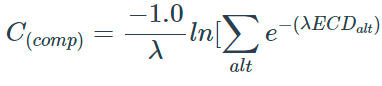
Where:
C(comp) is the composite cost
![]() is a scale parameter
which reflects the travelers sensitivity to cost differences
is a scale parameter
which reflects the travelers sensitivity to cost differences
ECDalt is the expected (generalized) cost to destination via a particular alternative
At choices between transit alternatives, the process computes the cost to the destination by adding the cost of the transit leg (including boarding and transfer penalties) and the expected cost to the destination from the end of the transit leg. Then, the process combines the values for the transit alternatives into a single value for the expected cost from the node to the destination. This is calculated as the average of the costs associated with each alternative (weighted by the probability of passengers taking the alternative).
In calculating the transit element of the expected cost to destination, the process applies an additional condition to ensure that adding (or improving) services does not increase costs. Specifically, the process examines each service operating between a pair of boarding and alighting points and includes the service if the resulting reduction in wait time exceeds the resulting increase in travel time. The process ensures that the expected time to the destination from the boarding node improves when a service is included in the set of attractive alternatives. This set of services is known as the basic choice set.
Models applied at decision points
This section describes the mathematical models that calculate the conditional probabilities for choices made at a route’s decision points. Models are available for cases where there are:
The route-evaluation process applies the walk-choice model when passengers have alternative walk choices available. For example, when passengers leave the origin or alight from a service, they might walk to their destination, board a different line at that stop, or walk to another stop for the next transit leg.
This model has a logit structure:
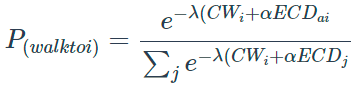
Where:
P(walktoi)is the probability of walking to boarding stop i
![]() is the scaling factor
for the model (LAMBDAW)
is the scaling factor
for the model (LAMBDAW)
CWi\) is the walk (generalized) cost to the boarding stop i
 is the cost weighting factor
(between 0 and 1), specified by
ALPHA. A value of 1 indicates that the walk and onward
costs have equal weight; lower values indicate that the walk cost has more
influence than onward cost in the traveller’s choice. For example, a
traveller’s willingness to walk may relate to familiarity with the network.
is the cost weighting factor
(between 0 and 1), specified by
ALPHA. A value of 1 indicates that the walk and onward
costs have equal weight; lower values indicate that the walk cost has more
influence than onward cost in the traveller’s choice. For example, a
traveller’s willingness to walk may relate to familiarity with the network.
ECDi is the expected (generalized) cost to destination from i.
ECDj is the expected (generalized) cost to destination from j.
Composite cost adjustment for ALPHA
The difference between the average and composite cost values, calculated as part of any logit model, represents the value of choice, or the benefit travelers gain from choosing between available alternatives.
When the ALPHA value that the walk-choice model uses is less than 1.0, the cost from the end of the walk leg to the destination is discounted. The composite-cost specification, shown above, represents the true cost to the destination (or trip cost), and has a different numeric value from the discounted form.
To adjust for an ALPHA value less than 1.0, the process estimates a composite cost consistent with the nondiscounted cost to the destination. First, the process uses ALPHA to calculate the value of choice for the walk-choice model. Next, the process subtracts this value of choice from the average cost (evaluated with ALPHA set to 1.0) to estimate the nondiscounted (true) composite cost.
The scaling factor LAMBDAW controls the shape of the logit curve used to allocate passengers to alternatives at each decision point. Large the scaling factors produce a smaller spread of trips between alternatives—that is, more trips are allocated to the best route. Conversely, low scaling factors produce trips spread over a wider range of alternatives.
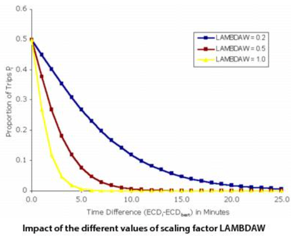
The X-axis shows the difference between the time by service i, ECDi, and the time by the best service, ECDbest. The Y-axis shows the proportion of trips allocated to the longer choice when a binary choice is available. The diagram plots three different values for the scaling factor: 0.2, 0.5, and 1. The curve for LAMBDAW = 0.5 shows that a choice five minutes longer than the best would be allocated 7.6% of the total trips. With a scaling factor of 0.2, the longer route gets 26.9% of trips, but with a scaling factor of 1.0, the longer route gets only 0.67% of trips. Thus, longer routes get a larger share of the trips as the scaling factor is reduced.
Two models are available to allocate passengers to the transit choices available at a stop: the service-frequency model (SFM) and the service-frequency-and-cost model (SFCM). SFM considers only service frequency while SFCM also considers the cost to the destination. See SFM and SFCM examples for examples that show how the two models treat transit choices at a stop.
Service-frequency model
Applied at stops with a basic set of transit choices, the service- frequency model calculates the conditional probabilities of the individual lines in proportion to their frequency. The model is equivalent to travelers who arrive randomly without knowledge of the timetables and take the first reasonable service forward from the node.
Where:
PuserlineI is the probability of using line l.
FrequencylineI is the frequency of line l (in services per hour).
FrequencylineK is the frequency of line k (in services per hour).
Service-frequency-and-cost model
The service-frequency-and-cost model is an extension of the service-frequency model. The model assumes that travellers have knowledge of the travel time to the destination associated with each of the alternative routes, and that the traveller is less willing to use slower alternatives. This model defines its own set of transit choices, which may be different from the basic choice set described in Deriving cost used.
To define a set of transit choices, the model selects the line with lowest expected cost to the destination. Next, the model considers the next fastest line. If that line passes the validity test, the model adds the line to the set of selected lines and repeats the process, considering the next fastest line. Once a line fails the validity test, the process terminates and the model uses the set of lines currently selected as possible routes to the destination.
The validity test computes the line’s "excess time" — the difference between its time to destination and the average value for the lines already selected (excluding wait time at the stop). The test compares the line’s excess time to the expected cost of waiting (which is based on the headway of the combined services already selected, and any wait factors):
-
If the excess time has a value of zero (that is, the line is no slower than those already selected), then the line is always a valid choice.
-
If the excess time is more than the expected cost of waiting, then the line is not valid; travellers are better off ignoring this line and waiting for the next service from the selected set.
-
If the excess time is greater than zero but no more than the expected cost of waiting, the line is valid some of the time. Specifically, excess time divided by the cost of waiting defines the proportion of time that travellers are better off ignoring the line. Therefore, one minus this proportion defines the probability of using the line when its service arrives at the stop.
As the probability of use varies between lines, the frequency of the combined services takes account of probability of use, as follows:
where:
P(use l) is the probability of using line l when a service is at the stop.
Frequency(line l) is the frequency of the line l (in services per hour).
Frequency(combined) is the combined frequency of a set of selected lines (in services per hour).
During loading, the proportion of demand using a particular line is given by:

The route-evaluation process applies the alternative-alighting model when a line has two or more valid alighting points. This model has a logit structure similar to the walk-choice model:

P(alight at i) si the probability of alighting at stop i.
![]() is the scaling factor
for the model (LAMBDAA).
is the scaling factor
for the model (LAMBDAA).
Note: LAMBDAA affects the choice of alighting points just as LAMBDAW affects walk choices. For an example, see Impact of the different values of scaling factor LAMBDAW.
ECDi is the expected (generalized) cost to destination via alternative alighting point i.
ECDj is the expected (generalized) cost to destination via alternative alighting point j.
At transfer points between transit services, the route-evaluation process applies a combination of models. First, the walk-choice model allocates demand between true walk alternatives and an imaginary alternative that represents the transit services available at the node. Next, the service-frequency model allocates the transit demand to the various services at the stop.
This section provides examples of the service-frequency model and the service-frequency-and-cost model:
Example of the service-frequency model
This example shows:
| (1) Line | (2) Travel Time | (3) Frequency | (4) Cum Frequency | (5) Wait Time | (6) Cum Travel Time | (7) Average Travel Time | (8) Travel + Wait Times | (9) Include Line |
|---|---|---|---|---|---|---|---|---|
| 1 | 20 | 5 | 5 | 12.0 | 100 | 20 | 32.0 | Y |
| 2 | 21 | 6 | 11 | 5.455 | 226 | 20.545 | 26.0 | Y |
| 3 | 22 | 2 | 13 | 4.615 | 270 | 20.769 | 25.385 | Y |
| 4 | 24 | 1 | 14 | 4.286 | 294 | 21 | 25.286 | Y |
| 5 | 26 | 1 | 15 | 4.0 | 320 | 21.333 | 25.333 | N |
Notes:
-
Lines 1-4 are included in the basic choice set because, with the addition of each line, the overall time to destination improves. Line 5 is excluded from the basic choice set because including it makes the time to destination worse.
-
A wait factor of 2 was used to weight the waiting times.
-
Column (5) = 60.0/(4) * 0.5 * Wait Factor
-
Column (6) = (2)*(3), accumulated over lines
-
Column (7) = (6)/(4)
-
Column (8) = (7)+(5)
Results of the service frequency model
Notes:
Column(4) = (2)/cumulative frequency at stop
Example of the service-frequency-and-cost model
This example shows:
| (1) Line | (2)Frequency | (3) Travel Time | (4) Average travel time excluding this line | (5) Excess travel time over average | (6) Wait time without this line | (7) Proportion of time when line used | (8) Cum effective frequency | (9) Wait time including this Line | (10) Average travel time including this line |
|---|---|---|---|---|---|---|---|---|---|
| 1 | 5 | 20 | - | - | - | 1 | 5 | 12 | 20 |
| 2 | 6 | 21 | 20 | 1 | 12 | 0.917 | 10.500 | 5.714 | 20.52 |
| 3 | 2 | 22 | 20.52 | 1.48 | 5.714 | 0.742 | 11.983 | 5.007 | 20.707 |
| 4 | 1 | 24 | 20.707 | 3.293 | 5.007 | 0.342 | 12.326 | 4.868 | 20.798 |
| 5 | 1 | 26 | 20.798 | 5.202 | 4.868 | 0 | - | - |
Notes:
-
Example uses a wait factor of 2 to weight the waiting times.
-
Column (4) = (10) from the previous line
-
Column (5) = (3) - (4)
-
Column (6) = (9) from the previous line
-
Column (7) = 1-MIN( (5)/(6)),1)
-
Column (8) = (2)*(7), accumulated over lines
-
Column (9) = 60.0/(8) * 0.5 * Wait Factor
-
Column (10) = ((2)*(3)*(7), accumulated over lines) / (8)
Results of the service frequency & cost model
Notes:
-
Column (3) = (2) * Proportion of time when line used (values are listed in Column (7) in the Choice set table above)
-
Column (4) = (3), accumulated over lines
-
Column(5) = (3)/cumulative frequency at stop
The skimming process extracts the cost of a public transport trip into a zone-to-zone matrix.
Because the Public Transport program finds multiple routes between zone pairs, the program can provide several skims, suitable for different purposes:
-
Composite-cost skim — Supports scheme evaluation and demand modeling
-
Value-of-choice skim — Indicates the choice available in the public transport system
-
Average skims — Supports model validation, operational statistics, revenue calculation
-
Best-trip skim — Indicates actual trip cost
Available skims and the processes for extracting them are described in Skimming (level of service) and Skim functions — quick reference.
For each zone pair, the composite-cost skim computes the composite cost, or the total utility of the trip including the choices available to the traveller.
The route-evaluation process uses composite costs, also referred to as the expected cost to destination (see Deriving cost used for a description of how they are derived).
To enable you to model demand or evaluate schemes, the skim ensures that adding new routes or improving services does not lead to an increase in the cost.
The skim calculates composite costs from each decision point in the trip to the destination. The calculation varies with the type of choice:
For each zone pair, the value-of-choice skim computes the value of choice, a measure of the extent to which travellers can choose between alternative routes. Higher values indicate travellers can choose between routes of similar costs, whereas lower values indicate a lack of route choice, or choices where the lesser alternatives are considerably more expensive than the best route.
The value of choice provides a measure of the resilience or robustness of the public transport system. With more low-cost choices, the system can continue functioning following the failure of one or more components.
The value-of-choice skim is equivalent to the difference between the composite-cost skim and the average-generalized-cost skim.
Average skims compute the costs a typical traveller incurs while making a public transport trip. You can extract average skims for all components of the trip. There are three broad areas:
Because multiple routes might connect zone pairs, average skims weighting each route according to its probability of use.
Average skims compute component costs at network and route-set level. Within each route set, average skims can compute costs other than wait time by mode.
Several average skims can compute either actual values—true measures of the cost—or perceived values—the cost’s contribution to generalized cost (usually a product of the cost and a weighting coefficient).
Average skims are appropriate for model validation and skimming operational statistics, such as passenger miles, hours, and revenue.
For each zone pair, the best-trip skim computes the actual time for the best route (that is, the time if travellers make the best choice at every decision point).
Because the skim uses actual values for all trip components, the skim does not reflect traveller behavior, and is, therefore, inappropriate for demand modeling.
The skim bases the wait time and the transit-leg time on the lowest expected values. The skim computes wait times from the appropriate wait curve, using the combined frequencies of all acceptable lines from the node towards the destination. The skim computes transit-leg times from the fastest line in the leg-bundles used.
Note: At present, walk (nontransit) legs have only one time attribute, the one used to construct them (perceived time). See Walk time (nontransit time).
The loading process (assignment) allocates trips, either computed or from the input trip matrix, to services (transit lines) and nontransit legs. The loading process uses routing and travel time information obtained from the route-evaluation process.
The loading process considers one origin-destination zone pair at a time. The process assigns the zone pair’s trips to the available routes according to each route’s probability of use, calculated during the route-evaluation process.
For example, consider the reports of enumerated and evaluated routes between zones 1 and 3.
Enumerated routes between zones 1 and 3
REnum Route(s) from Origin 1 to Destination 3
1 -> 773
773 -> 764 -> 764 lines GMB1-24MB
764 -> 751 -> 751 lines PLB1-113B PLB129B PLB127A
751 -> 749 -> 3 lines GMB1-2B
Cost=27.668
1 -> 773
773 -> 759 -> 759 lines GMB1-24MB
759 -> 875 -> 875 lines RES34R
875 -> 749 -> 3 lines GMB1-2B
Cost=34.028
1 -> 2052
2052 -> 2004 -> 875 lines ISL-DN
875 -> 749 -> 3 lines
GMB1-2B
Cost=31.84
Evaluated routes between zones 1 and 3
REval Route(s) from Origin 1 to Destination 3
1 -> 773
773 -> 764 -> 764 lines GMB1-24MB
764 -> 751 -> 751 lines PLB1-113B PLB129B PLB127A
751 -> 749 -> 3 lines GMB1-2B
Cost= 23.668 Probability=0.631438
1 -> 773
773 -> 759 -> 759 lines GMB1-24MB
759 -> 875 -> 875 lines RES34R
875 -> 749 -> 3 lines GMB1-2B
Cost= 28.628 Probability=0.142594
1 -> 2052
2052 -> 2004 -> 875 lines ISL-DN
875 -> 749 -> 3 lines GMB1-2B
Cost= 30.04 Probability=0.225968
The first report shows three bundles of enumerated routes from zone 1 to zone 3. All routes meet the evaluation criteria; none are eliminated. The second report lists the routes with their probability of use. The enumerated-routes report shows used costs. However, the evaluated-routes report shows the average cost for the route bundle, not the composite costs used to calculate the probability of use.
The loading process considers two walk choices from zone 1: to nodes 773 and 2052. The route-evaluation process determined that the probability of going to node 773 is 0.774032, while the probability of going to node 2052 is 0.225968, reflecting the shorter time via node 773. The loading process splits trips from zone 1 to zone 3 in this proportion and saves the trips for the nontransit (access) legs:
-
At node 773, there is a single transit service, GMB1-24B; all trips arriving at node 773 board this service. There are two alighting points: nodes 764 and 759. The time via 764 is less than the time via 759. Thus the probability of using node 764 is 0.631438 and the probability of using node 759 is 0.142594. The loading process splits trips at node 773 between the two alighting points and saves the trips for the two transit legs.
-
At 764, the loading process assigns arriving trips to lines PLB1-113B, PLB129B, and PLB127A in proportion to their relative frequencies for trips to node 751. From node 751, travelers go to zone 3 via node 749 and line GMB1-2B. The process saves the number of trips assigned to the four transit legs for each leg.
-
At node 759, the loading process assigns arriving trips to transit lines RES34R and GMB1-2B for trips to nodes 875 and 749 before ending at zone 3.
-
-
At node 2052, the loading process assigns travelers to transit line ISL-DN for the trip to node 875, and then to transit line GMB1-2B for the trip to node 749 before ending at zone 3.
All trips from zone 1 to 3 use line GMB1-2B as the last transit leg in the trip, and alight at node 749 where they walk to zone 3. These are saved for the nontransit (egress) leg 749-3.
The loading process is complete after assigning trips between all (selected) origin-destination zone pairs, and computing the total trips using transit and nontransit legs on the underlying network links.
This section describes how to model fares in the Public Transport program. Topics include:
Fares are a fundamental element of a public transport trip. Therefore, it is important to incorporate fares fully into the Public Transport modeling process.
To incorporate fares, the Public Transport program:
-
Considers fares in the route choice
-
Skims average fares for each origin-destination zone pair
-
Calculates and reports revenue
Fares do not always significantly impact route choice. To reduce run times, you might exclude fares from the route-evaluation process and skim and calculate revenue from the evaluated routes.
The Public Transport program must accurately represent the fare systems that passengers face. The Public Transport program provides a framework which you can use to directly represent or approximate most fare systems. In fact, you can represent different types of fare systems within a single public transport network.
You can specify fare systems and value of time by user class. You might do this to use readily available ticket type data to segment and model demand by ticket type.
Transit legs are the basic unit the program uses to calculate fares. A transit leg is one part of a trip, from a boarding point to an alighting point, that uses a single transport line. The program assigns each line to a fare system, either directly or through its mode or operator.
The program calculates fare for a single leg of the trip. If multiple consecutive legs have the same fare system, the program assumes integrated or through ticketing and calculates fare for that sequence of legs.
To model fares, the Public Transport program requires a program- wide "fare system" that describes each transit line’s individual fare system, its data requirements, and how it interfaces with other lines.
You define fare systems with the FARESYSTEM control statement and input fare systems with the FILEI FAREI file. You define fare system attributes with FARESYSTEM keywords and subkeywords:
-
Unique numeric and character identifiers (NUMBER, NAME, LONGNAME)
-
Unit of measure for trip length, such as distance, number of fare zones crossed, or boarding-alighting fare zones. (STRUCTURE, with possible values: FLAT, DISTANCE, HILOW, COUNT, FROMTO, or ACCUMULATE)
-
Boarding costs at the initial boarding and subsequent transfers, and the cost of transferring between fare systems (IBOARDFARE, FAREFROMFS)
-
Trip cost, which may be specified with a coefficient per unit measure of the trip, a table, or matrix (UNITFARE, FARETABLE, FAREMATRIX)
-
Rules for computing costs when transferring to the same fare system and interpreting fare tables (SAME, INTERPOLATE)
Data requirements for fare systems depend upon the unit of trip measure (specified with STRUCTURE) and the method for specifying trip costs (specified with UNITFARE, FARETABLE, and FAREMATRIX). Requirements can vary from minimal to substantial. The following table provides a quick reference to the various fare systems and their data requirements.
| STRUCTURE | FLAT | DISTANCE | HILOW | COUNT | FROMTO | ACCUMULATE |
|---|---|---|---|---|---|---|
| IBOARDFARE | Required | Optional | Permissible | Permissible 3 | Permissible | Permissible |
| FAREFROMFS | Optional | Optional | Optional | Optional | Optional | Optional |
| UNITFARE | NA | Optional 1 | NA | NA | NA | NA |
| FARETABLE | NA | Optional 2 | NA | Required | NA | Required |
| FAREMATRIX | NA | NA | Required | NA | Required | NA |
| FAREZONE | NA | NA | Required | Required | Required | Required |
One of the two items is required.
One of the two items is required.
Permitted but use is questionable, as it could be included in the FAREMATRIX.
The program assigns fare systems to transit lines indirectly through the line’s mode and operator with the FACTORS FARESYSTEM keyword or directly with the LINE control statement. When modeling fares, each line must have an assigned fare system.
Include fares in the route-evaluation process by setting PARAMETERS FARE to T. Skim fares, whether or not they are included in route-evaluation, by selecting skimming functions FAREA and FAREP in the SKIMIJ phase.
The units for measuring trip-length is a key attribute of the fare system. Trip-length units might be based on legs, actual distance, or fare zones. Fare zones are single nodes or groups of nodes.
You specify the trip-length unit with the FARESYSTEM keyword STRUCTURE. There are six possible values. Each value results in a different method for calculating trip length and fare.
Description of trip-length units
-
FLAT - Trip length not used for fare calculation. Fares derived by leg using the boarding and transfer costs specified with IBOARDFARE and FAREFROMFS.
-
DISTANCE - Trip length measured as in-vehicle distance, in user-specified units.
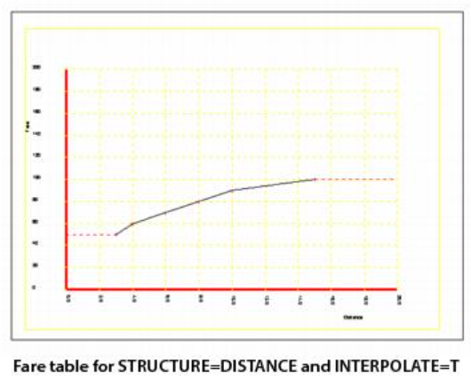
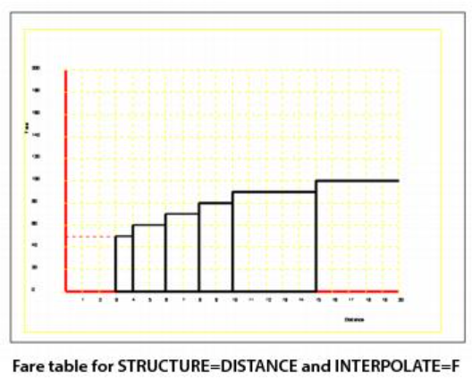
Fares calculated by leg or for sets of consecutive legs using the same fare system. Fares based on:
-
Boarding and transfer costs, specified with IBOARDFARE and FAREFROMFS.
-
Trip cost computed by multiplying in-vehicle distance by UNITFARE.
-
Trip cost obtained from the fare table specified by FARETABLE. The value of INTERPOLATE determines whether the program uses linear interpolation or a step function between coded points.
-
-
HILOW - Trip length measured by the highest and lowest fare-zones crossed.
Appropriate for an annular fare-zone structure.
Fares calculated by leg or for sets of consecutive legs using the same fare system. Fares based on:
-
Boarding and transfer costs, specified with IBOARDFARE and FAREFROMFS (boarding costs are added to the fare matrix)
-
Trip cost, extracted from the fare matrix specified with FAREMATRIX (rows contain the lower fare zone, and columns contain the higher fare zone)
-
-
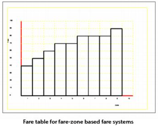
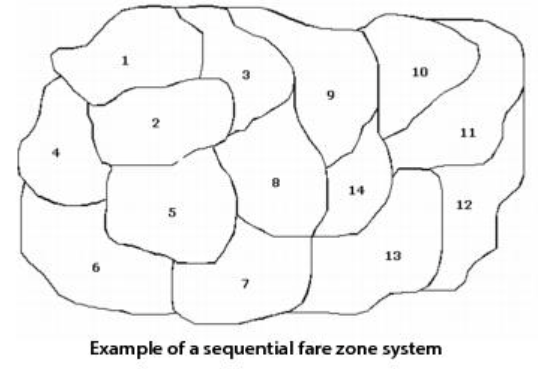
COUNT - Trip length measured by the number of fare zones crossed plus 1 for the initial zone.
Best suited to a sequential zone system.
Fares calculated by leg or for sets of consecutive legs using the same fare system. Fares based on:
-
Boarding and transfer costs, specified with IBOARDFARE and FAREFROMFS
-
Trip cost, extracted from the fare table specified with FARETABLE. In this case, the program interpolates the fare table as a step function.
-
-
FROMTO - Trip length measured as function of the boarding and alighting fare zones.
Best suited to a sequential zone system.
Fares calculated by leg or for sets of consecutive legs using the same fare system. Fares based on:
-
Boarding and transfer costs, specified with IBOARDFARE and FAREFROMFS (boarding costs are added to the fare matrix).
-
Trip cost, extracted from the fare matrix specified with FAREMATRIX (rows contain the lower fare zone, and columns contain the higher fare zone)
-
-
ACCUMULATE - Trip length measured by accumulating fares associated with each fare zone traversed. Differs from COUNT, where program counts the number of fare zones traversed to compute fare.
Best suited to a sequential zone system.
Fares calculated by leg or for sets of consecutive legs using the same fare system. Fares based on:
-
Boarding and transfer costs, specified with IBOARDFARE and FAREFROMFS
-
Trip cost, extracted from the fare table specified with FARETABLE. The fare table has a fare for each fare zone in the system.
-
For public transport networks with multiple fare systems, use the SAME subkeyword to specify whether the program treats consecutive legs in the same fare system as one leg or as separate legs when calculating fares.
If two consecutive legs of a trip use different fare systems, the program always calculates the fare separately for each leg.
Boarding and transfer costs are key attributes of the fare system. You specify boarding and transfer costs with FARESYSTEM keywords:
-
IBOARDFARE — Fare incurred upon boarding the first transit leg of a trip. See IBOARDFARE.
-
FAREFROMFS — Fare incurred when transferring from lines using other defined fare systems. See FAREFROMFS.
Trip cost is a key attribute of the fare system. The program determines trip cost using one of three methods:
-
UNITFARE — Coefficient used to calculate fares. Only available when STRUCTURE is DISTANCE. To obtain fare, the program multiplies UNITFARE by in-vehicle distance of a leg or a sequence of consecutive legs using the same fare system.
-
FARETABLE — Table of fares. Used when STRUCTURE is DISTANCE, COUNT, or ACCUMULATE. Define FARETABLE with a list of paired X and Y coordinates, where X is the trip length and Y is the fare.
See FARETABLE for more information about coding FARETABLE. Some graphic examples follow.
-
FAREMATRIX — Matrix of fares. Used when STRUCTURE is HILOW or FROMTO. Input matrices with FILEI FAREMATI in either standard CUBE Voyager binary matrix format or as text records. See FAREMATRIX for information about coding fare matrices. To report on fare matrices, use the REPORT keyword FAREMATI.
You code fares in monetary units. The program converts fares to generalized costs using the FACTORS keyword VALUEOFTIME.
Fare systems that have the STRUCTURE set to HILOW, FROMTO, COUNT, or ACCUMULATE require fare zones. Fare zones are either groups of nodes or single nodes.
A public transport network might have multiple fare-zone schemes, but a fare system must have only one zone scheme. Therefore, a node can be in only one fare zone.
The HILOW structure requires an annular fare zone system while the other structures require sequential fare zones.
To identify and code fare zones for fare systems with a FROMTO, COUNT, or ACCUMULATE structure
-
Display the network in CUBE.
-
Add a new node attribute to store the fare zone, such as FAREZONE.
-
Use the Polygon menu to define fare zones, one at a time
-
Assign a number to the new fare-zone attribute of the nodes within the polygon
To identify and code fare zones for fare systems with a HILOW structure
-
Display the network in CUBE.
-
Add a new node attribute to store the fare zone, such as FAREZONE.
-
Associate the number of the outermost fare zone to the new fare-zone attribute of all nodes.
-
Use the Polygon menu to define a ring separating the outermost fare zone from the other zones.
-
Assign the number of the penultimate fare zone to the new fare-zone attribute of the nodes within the polygon
-
Repeat the last two steps until all fare zones have been completed.
This section shows how fares are calculated for a four-leg trip using different fare models, individually and in combination.
Example 1: FLAT fare system
FARESYSTEM NUMBER=1, NAME=Flat Fare British Rail’, STRUCTURE=FLAT,
IBOARDFARE=100, FAREFROMFS[1]=0, 100
FARESYSTEM NUMBER=2, NAME=Flat Fare Underground+Bus’, STRUCTURE=FLAT,
IBOARDFARE=50, FAREFROMFS[1]=75, 0
FACTOR FARESYSTEM=1, MODE=1
FACTOR FARESYSTEM=2, MODE=2,3
FARE(A-E) = 175 pence, which is the sum of fares for each leg, calculated as:
Leg A-B = 100 {IBOARDFARE for A-B} +
Leg B-C =  75 {FAREFROMFS[1] for B-C, for transferring from FARESYSTEM 1 to 2}
Leg C-D =   0 {FAREFROMFS[2] for C-D, for transferring from FARESYSTEM 2 to 2}
Leg D-E =   0 {FAREFROMFS[2] for D-E for transferring from FARESYSTEM 2 to 2}
Example 2: DISTANCE fare system
The trip uses three fare models, all with STRUCTURE set to DISTANCE but with different unit cost for trip length.
FARESYSTEM NUMBER=1, NAME=’Distance British Rail’, STRUCTURE=DISTANCE,
IBOARDFARE=100, FAREFROMFS[1]=0, 100, 100, FARETABLE=1.0,0.75, 5.0,2.50,
10.0,3.50
FARESYSTEM NUMBER=2, NAME=’Distance Underground’, STRUCTURE=DISTANCE,
SAME=CUMULATIVE, IBOARDFARE=100, FAREFROMFS[1]=100, 0, 100, UNITFARE=60
FARESYSTEM NUMBER=3, NAME=’Distance Bus’, STRUCTURE=DISTANCE,
IBOARDFARE=50, FAREFROMFS[1]=50, 50, 0, UNITFARE=50
FACTOR FARESYSTEM=1, MODE=1
FACTOR FARESYSTEM=2, MODE=2
FACTOR FARESYSTEM=3, MODE=3
FARE(A-E) = 950 pence, which is the sum of fares for trip legs, calculated as:
Leg A-B = 100 + 350 (IBOARDFARE + trip cost)
Legs B-D = 100 + (5*60) (FAREFROMFS[1] + total  distance * UNITFARE)
Leg D-E = 50 + (1*50) (FAREFROMFS[2] + total  distance * UNITFARE)
Note: Where two consecutive legs have the same fare system, the fare can be calculated for each leg separately or cumulatively, depending upon the setting of SAME. In this example, legs B-C and C-D have the same fare system and SAME is set to CUMULATIVE, so the fare is calculated for B-D. SAME has no effect in this case because UNITFARE is used rather than FARETABLE.
There is no cost for transferring from fare type 2 to another leg using the same fare type.
Example 3: FROMTO fare system
FARESYSTEM NUMBER=1, NAME=’Trip Based’, STRUCTURE=FROMTO,
FAREMATRIX=FMI.1.5, FAREZONES=NI.FAREZONE
FACTOR FARESYSTEM=1, MODE=1-3
FARE(A-E) = 350 pence,
The node variable, NI.FAREZONE, defines the fare zones for stops A through E, and the program extracts the fare from fare matrix number 5, input on FAREMATI[1], row NI.FAREZONE(A) and column NI.FAREZONE(E).
There are no boarding costs or costs for transferring between the same fare system.
Example 4: COMBINATION of FROMTO and DISTANCE fare systems
The two FROMTO fare systems use different FARETABLE values and an incentive is offered to interchange between fare system 1 and 2 and vice versa.
FARESYSTEM NUMBER=1, NAME=’British Rail’, STRUCTURE=FROMTO,
FAREMATRIX=FMI.2.BritRail, FAREFROMFS[1]=0, -25, 0, FAREZONES=NI.FAREZONE
FARESYSTEM NUMBER=2, NAME=’Underground’, STRUCTURE=FROMTO,
SAME=CUMULATIVE, FAREMATRIX=FMI.1.UndGrnd, FAREFROMFS[1]=-25, 0, 0,
FAREZONES=NI.FAREZONE
FARESYSTEM NUMBER=3, NAME=’Bus’, STRUCTURE=DISTANCE, UNITFARE=50,
IBOARDFARE=50, FAREFROMFS[1]=50, 50, 0
FARE (A-E) = 525 pence, which is the sum of fares for legs, calculated as:
Leg A-B = 250 (FAREMATRIX FMI.2.BritRail, row NI.FAREZONE(A), column
NI.FAREZONE(B))
Leg B-D = -25+200 (FAREFROMFS[1] and FAREMATRIX FMI.1.UndGrnd, row
NI.FAREZONE(B), column NI.FAREZONE(D))
Leg D-E = 50 + 1*50  (FAREFROMFS[2] + trip cost)
An iterative process, crowd modeling enables a public transport system’s capacity to influence the system’s travel times and thus the routes found and their probability of use, as calculated during route evaluation. The Public Transport program supports two types of crowd models:
This section also discusses:
A link-travel-time adjustment models a passenger’s perception that travel time is more onerous when standing (rather than sitting), or when in crowded vehicles. Specify this adjustment with a "crowding factor". The program multiplies the crowding factor by in-vehicle time to determine the perceived "crowded in-vehicle time".
For example, suppose a vehicle has a seating capacity of 40, crush capacity of 50, and load distribution factor of 0.85 (standing occurs when more than 85% of 40—that is, 34 seats—are occupied). Once standing starts, the crowding factor might increase slowly from 1.0 for the first few standing passengers, then more steeply once vehicle loading exceeds 40.

The Public Transport program uses crowding curves. Derived from the crowd-factor curve, crowding curves show utilization on the X-axis. Utilization, the percentage of standing places occupied, can vary between 0 and 100with the default option, but a user control keyword UTFLEX allows to specify crowding curves for values of Utilization beyond 100%. The corresponding crowding curve is shown below.

Crowd factors are 1.0 in uncrowded conditions, and typically rise to values in the ranges 1.0 to 1.4 for seated passengers and 1.5 to 3.0 for standing passengers when the vehicle is fully loaded with standing occurring.
The program calculates crowded link travel time as:
where:
Tc is the crowded link travel time
Tu is the link travel time (in uncrowded conditions)
CCrvv,c(U) is the crowd curve value (where the curve is specific to a vehicle type, v, and a user class, c) for utilization U
U is the utilization measure (as a percentage)
The utilization measure (as a percentage), U, is defined by the expression:
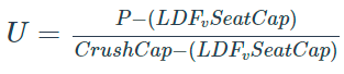
where:
P is the passenger demand (per hour).
SeatCap is the seating capacity (per hour) for the line.
CrushCap is the crush capacity (per hour) for the line; this is the total of seated and standing capacities.
With the default settings, the value of utilization is constrained with a minimum value of 0% (when no standing occurs) and an upper limit of 100% (when crush capacity is exceeded). A user selected keyword UTFLEX allows to specify utilization values beyond 100%.
If the values of seating capacity and crush capacity are identical for any line, then utilization is 100% whenever demand exceeds the seating capacity, and 0% otherwise.
The wait-time adjustment reflects the ability to board a service. In simple models (without crowd modeling) travellers typically board the first service that arrives at a stop and goes to the required alighting point. As loadings on services increase, this becomes less realistic, as travellers will choose the first appropriate service that has available capacity. Using measures of demand and available capacity, the wait-time adjustment computes the probability of being able to board a service. With heavily loaded services, some travellers will wait for the next service, incurring additional wait time at the boarding node.
Without crowding, the program assigns demand with the service- frequency model (SFM), or service-frequency-and-cost model (SFCM). The wait-time adjustment redistributes the initial SFM or SFCM loadings whenever any line does not have the available capacity to take its assigned demand. The program reassigns this excess demand to other lines with spare unused capacity; those travellers incur additional wait time.
The additional wait time might make this route less attractive, resulting in diversion of demand to other enumerated routes for the origin-destination pair.
If demand exceeds capacity and no alternative routes are available, then this transit leg acts as a "bottleneck"—not all of the travel demand is able to use the service during the modeled period. The demand remaining at the end of the modeled period would discharge once peak travel volumes subside; those travelers experience additional delays, which form a second component to the wait-time adjustment.
"Flow metering" handles the bottleneck effect and the inability of demand to pass through that point. Flow metering removes the excess demand from later stages in the trip; thus demand at any downstream point reflects the number of travellers who can reach that point. For any origin-destination pair, the program can calculate the proportion of flow-metered demand (that is, demand unable to reach its destination due to network bottlenecks), and the number of trips affected.
The crowd modeling process uses the loaded demand from an iteration to provide updated values for:
-
Link travel times (which may vary by user class)
-
Probability of being able to board a line at a particular stop
These calculations incorporate a degree of damping to help stabilize the resulting assignments.
All damping factors work in the EMA type formula, i.e., X(new) = X(old) + LINKDF/VOLDF/WAITDF *(X(calculated) – X(old)). Where X corresponds to crowding factors, crowding volumes, capacity and demand averaging, for LINKDF, VOLDF, WAITDF respectively. Higher damping factors implies higher weights to the most recent (calculated in the current iteration) X values, whilst lower damping factors implies higher weights for averaged X values from the previous iteration.
The crowding process is viewed as a stochastic assignment, and results are obtained from the final iteration.
Crowded networks might cause instabilities in the loadings between iterations, as demand switches toward less congested routes. In turn, those routes might become more heavily loaded, and thus less attractive at the next iteration. These changes might converge toward a solution, or might continue oscillating; oscillation is more likely in highly overloaded networks. The service-frequency-and-cost model usually results in better convergence than the service-frequency model because the route- choice process is more responsive to changes in costs.
Four keywords can be used to impose automatic stopping criteria to this iterative process (RMSESTOP, RMSECUTOFF, RDIFFSTOP and RDIFFCUTOFF). If the stopping criteria are unset or not met, the program will stop at the iteration specified by the ITERATIONS keyword.
The formulas used to calculate these iteration-by-iteration statistics are reported below:
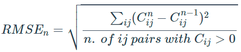
Where:
C = Composite Cost
n = Current iteration number
ij = OD pair
u = User class
The crowding algorithm will run one extra iteration after the stopping criteria are met for three consecutive iterations, and output the corresponding results. This behaviour (one more step to stop) is due to the original design of the PT process, based on a predefined maximum number of iterations as stopping criteria.
Due to the heuristic nature of the Public Transport crowding algorithm, this stopping criteria that the program provides should not be considered a convergence measure. Therefore, it is suggested that users also analyse the evolution of the assignment algorithm iteration-by-iteration, using the statistics and measures provided by the other available keywords (RDIFF, REPORTIJ, RMSE, SKIMS, STOP2STOP and TRACEIJ).
The Public Transport headway-based approach assumes that travelers arrive at a stop at random and take the first service available. The headway-based model is suitable for modeling urban areas with high frequency services and/or with complex public transport systems. Both initial and transfers Wait Time are a function of the service frequencies, that can be customized by the user.
PT's timetable-based, or timetabling, model uses the actual timetable for services as its basis, and it is appropriate for smaller systems, when services are infrequent but regular, or when connections between services need to be coordinated (e.g. bus feeders to rail services). Within this approach, travelers are assumed to have comprehensive knowledge of the service timetable. Therefore, initial Wait Time is assumed to be zero, and transfers Wait Time has fix values calculated by the program based on services arrival and departure times.
Timetable-based modeling needs a different approach in describing the Public Transport services, with different keywords, then a headway-based model. The program structure and files content are similar.
This section describes:
Line File keywords
The Line File describes the available services with a structure similar to the structure of the headway-based approach. Nevertheless, the following additional keywords need to be specified for each single line.
- DAYTYPE - List of numerical values representing the day types on which the specific line operates (e.g. 1=Weekday, 2=Saturday and 3=Sunday). The list is required, and no default is provided. The lines to operate are then selected by the value of the same keyword specified in the Factor File.
- RUNINTERVAL - Defines the headway in minutes between departures of the services from the first/starting node of the line. RUNINTERVAL is used only when the STARTTIMES are given as ranges. The RUNINTERVAL value refers to the STARTTIMES range immediately following it.
- STARTTIMES - Defines a list of departure times of services running from the first/starting node of the line. The values can be specified in two formats (also using a combination of the two):
For example, the two specifications below for the "Bus_1" line results in the same services.
Example using individual STARTTIMES.
LINE NAME="Bus_1",
MODE=1,
ONEWAY=T,
DAYTYPE=1,
STARTTIMES=0700,0720,0740,0800,0830,0900,
N=106,
N=141, RT=10,
N=162, RT=40
Example using combination of RUNINTERVAL with STARTTIMES ranges and individual STARTTIMES.
LINE NAME="Bus_1",
MODE=1,
ONEWAY=T,
DAYTYPE=1,
RUNINTERVAL=20, STARTTIMES=0700-0800,
STARTTIMES=0830,0900,
N=106,
N=141, RT=10,
N=162, RT=40
Factor File keywords and path building process
The Factor File allows to specify most of the keywords used with the headway-based approach, but the following additional keywords are available for timetabling.
- DAYTYPE - The day type number to which the model relates. This selects the lines which operate on that day type.
- PERIOD - Range of values in hhmm-hhmm format which specify start and end of modeled period. E.g., PERIOD=0930-1029 means that the period goes from 09:30AM to 10:29AM and the services that are running in this period include all the services with STARTTIMES included in this range, with travelers leaving the origin within this period (including the start and end times, i.e., [09:30-10:30]). When PERIOD is specified, the program simulates the entire time interval, with a uniform distribution of trips for the entire period. There is no default value.
- •TIMEPOINT - This is an alternative to PERIOD to specify the departure time for the modeled trips. The traveler leaves the origin at this fixed/defined time (specified in hhmm format) and appropriate paths are found and evaluated. E.g., TIMEPOINT=1015 means that the trips are leaving the origin centroid at 1015. It is possible to have (up to 10) different user classes within the same PT program, each one with a different matrix, associated to different TIMEPOINTs. Also, for this keyword there is no default value.
As mentioned above, zero initial Wait Time is considered by the model, assuming travelers arriving just-in-time for the initial departure. Transfers Wait Time, instead, is calculated based on the arrival time of the first line and the departure time of the subsequent line, subtracting any NT transfer time between arrival and departure stop nodes. The following keywords allow to impose additional conditions to the transfers Wait Time in the Factor File and by node in the input network:
- • MINXFERVAR - This specifies the name of a node variable (defined in the input network node attributes) which holds the user-imposed minimum wait time when undertaking a transfer at the node (excluding the NTLEG, if applicable). When interchanging at a node, the departure time must be later than the arrival time plus this minimum wait time, therefore representing the minimum total transfer time at that node. Specifying "varName" will result in using "ni.varName" from the input network.
- • MAXWAITVAR - Specifies the name of a node variable (defined in the input network node attributes) which holds the maximum wait time travelers are prepared to spend waiting at each transfer node. When interchanging at a node, the departure time cannot be later than the arrival time plus the maximum wait time, therefore representing the maximum total transfer time at that node. Specifying "varName" will use "ni.varName" from the input network.
The "best path" concepts for the timetable-based approach are different than for the headway-based approach. Four different path building methodologies are available in timetable-based modeling. These are triggered depending on the value of the below three keywords (multipaths is implemented when the three keywords are set to False, which is also their default value).
- QUICKESTPATH - When set to true, enumerates one single fastest path for a departure time for each origin to destination. No route enumeration criteria are applied. XFERPEN penalties are considered. Default is False.
- QUICKESTMULTI - When set to true, enumerates one single fastest path for multiple departure times for each origin to destination (note that the same departure time is enumerated just once). Route enumeration criteria are applied. XFERPEN penalties are considered. Default is False.
- BESTPATHS - When set to true, enumerates multi-routing (i.e., multiple paths for each departure time), then selects the lowest generalized cost path for each departure time, representing the best paths for the Origin Destination pair. If BESTPATHS is False (default), full multi-routing takes place ("MULTIPATHS"), enumerating multiple paths for each departure time and each path is included in route evaluation (calculation of probabilities). In both cases XFERPEN penalties are not considered.
If multi-routing process is implemented, choice probability is calculated based on the Generalized Cost for the entire path, rather than at each single decision point as in the headway-based evaluation process. One of two models (Kirchoff and Logit) can be chosen for the choice probability calculation as explained below.
- KIRCHOFF - When set to true, uses the Kirchoff power-function to determine choice probabilities. Requires the definition of the KBETA parameter. The default if False, implementing the LOGIT model instead.
- KBETA - Power used in KIRCHOFF distribution. Its value is coded positive but used as negative, e.g., KBETA=2 will calculate costs raised to the power -2. This parameter has no default value. The Kirchoff probability is given by the equation below for route r between the alternative routes (index t):
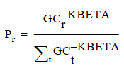
Where:
Pr= Probability of using route r
GCr= Generalized Cost for route r
- LAMBDAR - Scaling factor used with LOGIT model formulation for the calculation of probabilities. The default value is 0.2. The Logit probability is given by the equation below for route r between the alternative routes (index t):

Where:
Pr= Probability of using route r
GCr= Generalized Cost for route r
The System File structure is the same for headway-based modeling and timetable-based modeling. For timetable-based approach the definition of wait-curves is not needed, and if coded they will be ignored by the program.